\[ \renewcommand{\H}{\mathcal{H}} \newcommand{\tr}{\textnormal{tr}\,} \newcommand{\A}{\mathcal{A}} \newcommand{\Ac}{\mathcal{A}^*} \newcommand{\N}{\mathcal{N}} \renewcommand{\P}{\mathcal{P}} \newcommand{\Z}{\mathcal{Z}} \newcommand{\G}{\mathcal{G}} \newcommand{\D}{\mathcal{D}} \newcommand{\st}{\hspace{0.7mm}\textnormal{s.t.}\hspace{0.7mm}} \DeclareMathOperator*{\argmax}{arg\,max} \DeclareMathOperator*{\argmin}{arg\,min} \newcommand{\<}{\langle} \renewcommand{\>}{\rangle} \newcommand{\diag}{\textnormal{\textbf{diag}}} \newcommand{\eigs}{\textnormal{\textbf{eigs}}} \newcommand{\Diag}{\textnormal{\textbf{Diag}}} \newcommand{\T}{^\textsf{T}} \newcommand{\B}{\mathcal{B}} \newcommand{\Bc}{\mathcal{B}^*} \newcommand{\one}{\mathbf{1}} \renewcommand{\phi}{\varphi} \]
1 Quantum Key Distribution
To begin talking about quantum key rates, we must first talk about quantum cryptography and quantum encryption schemes. By now, most people have probably heard at some point “quantum computers are going to be able to hack secure information in a fraction of the time of classical computers", or”RSA encryption will be useless against quantum computers", or something of the like. And, although it will be a while before quantum computers are powerful enough to pose a real threat to current encryption schemes, it’s important to get ahead of the development and have quantum-safe encryption schemes ready to implement. Quantum key distribution (QKD) is just one of the many disciplines that provide a solution to the threat quantum computers pose to classical encryption (Broadbent and Schaffner 2016).
As in classical encryption, quantum encryption schemes use an encryption key to distort information so that eavesdropper can’t infer anything useful, and then use another key held by a trusted correspondent to decrypt the information. The discipline of quantum key distribution encompasses the creation of key distribution protocols, and the calculation of key rates for these protocols. QKD protocols are the processes used to create and distribute the keys between sender and receiver. To fully define a QKD protocol, you need to define the state of the qubits that Alice can prepare, methods Alice and Bob will use to measure the qubits, a potential third party Charlie to convey information to Alice and Bob, and the method through which Alice and Bob exchange information about their measurements (Winick, Lütkenhaus, and Coles 2018). To analyse a protocol, you need to define a model for environment noise, and an attack method for Eve to use - these determine the quantum channel.
To build a concrete understanding of what a QKD protocol encompasses, we will go through a simple protocol as an example, the BB84 protocol (named after its inventors Charles Bennett and Gilles Brassard (Bennett and Brassard 2014)). This description for this example is restated from Nielsen and Chuang Quantum Computation and Quantum Information (Nielsen and Chuang 2012).
The BB84 protocol is a type of “prepare and measure" protocol, another popular type of protocol is entanglement-based, where Charlie prepares an bipartite entangled state and sends one part to Alice and one to Bob. For this report we will focus on prepare and measure protocols.
We now move on to the second part of QKD: the computation of key rates for distribution protocols. The key rate is what quantifies how much usable secret key is distributed by a given protocol, it is the number of established secret key bits divided by the number of distributed quantum systems (number of qubits) (Coles, Metodiev, and Lütkenhaus 2016). Protocols with higher key rates are more desirable, so the ability to calculate a key rate for a distribution protocol is an important step in the development of new distribution protocols. Unfortunately (for quantum cryptographers, fortunately for me!) calculating the key rate is a pretty difficult problem. Devetak and Winter (2005) developed a formula for the key rate given known states of Alice, Bob, and Eve, but computing the key rate with those parameters specified only gives part of the picture. In order to be sure the protocol will work under all circumstances (all possible joint states of Alice, Bob, and Eve), a worst case key rate is computed. This is an optimisation problem whose solution lower bounds all possible key rates for a given protocol.
The rest of this section contains descriptions of some of the quantum information theory concepts discussed, which will hopefully provide some foundation for your thoughts. It concludes with some notation.
Measurement of quantum systems is characterized by projection operators. A projection operator is correlated with a measurement outcome, and the result of the measurement is the probability of obtaining said measurement outcome. Let’s say we have a projection operator \(P = \ket{00}\bra{00}\) corresponding to measurement outcome that both qubits are 0, then if we apply this to a state \(\rho = \frac{1}{4} \ket{00}\bra{00} + \frac{3}{4} \ket{10}\bra{10}\), the result is \(\frac{1}{4}\). Measurements can also be generalised to something called a positive operator-valued measure (POVM). A POVM is defined as a collection of positive semi-definite matrices \(\{P_i\}\) that sum to the identity
\[\sum_{i=1}^k P_i = I.\]
Each POVM element \(P_i\) corresponds to a measurement outcome indexed by \(i\), and the result of the measurement gives the probability of obtaining outcome \(i\)
\[\text{Prob}(i) = \tr(\rho P_i).\]
Projection measurements can be used to determine the density matrix of an unknown quantum system \(\sigma\). You can define the set of measurement operators to correspond to all possible states \(\{\ket{\phi_i}\}_{i=1}^n\) the system could exist in, then the outcome of the measurement is the probability \(p_i\) that the system is in state \(\ket{\phi_i}\). Let \(\sigma'\) denote the reconstructed system, it is defined as
\(\sigma' = \sum_{i=1}^n p_i \ket{\phi_i}\bra{\phi_i}.\)$
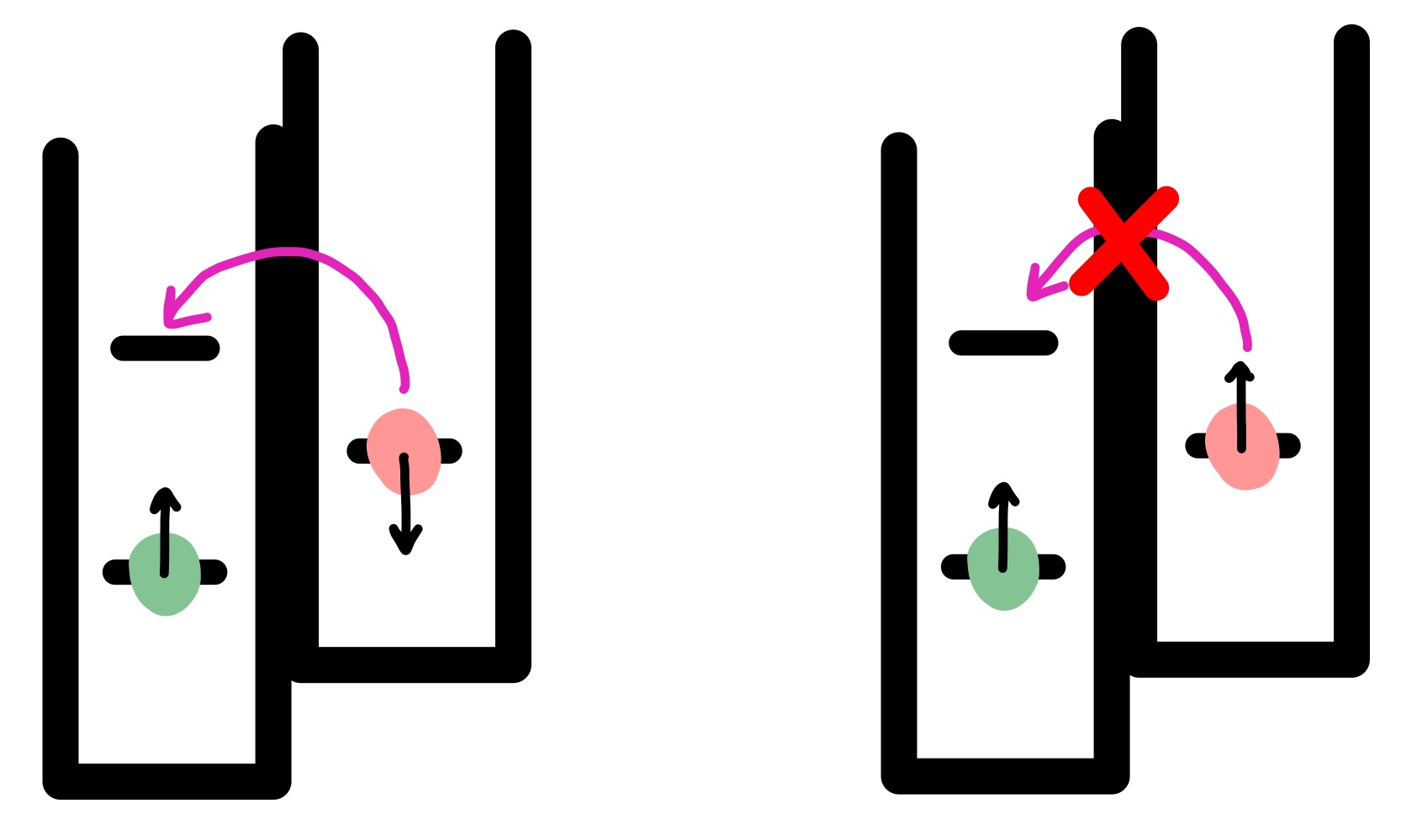
To provide the brain with something to hold onto while talking about “measuring” qubits, we describe, at a very high level, one method of doing so: spin selective tunnelling.
While it is possible to measure the spin of a quantum particle, it is time consuming - but most encryption protocols use spin qubits, meaning fast and reliable measurement is necessary. Spin selective tunnelling is a method to determine particle spin by measuring a charge (which is much faster to do). Suppose you have a qubit of known spin in a two state reservoir (remembering from chemistry that particles like electrons can have different activation states), next to this reservoir you have a different one state reservoir with a qubit of unknown spin. Quantum chemistry dictates that it is much harder for a particle with the same direction spin to tunnel to the left, but particles with opposite spin can tunnel much easier. When a particle tunnels and changes state, a small charge is emitted, and this is what is measured. Whether or not a charge is detected will determine if the measurement is taken to be a 0 or a 1 (based on the spin of the known qubit).
Information in this note was collected from Joe Salfi’s Introduction to Quantum Information and Computing course and Wikipedia (Salfi (2023),“Measurement in Quantum Mechanics” (2024)).
1.1 Notation
\(\H^n\) is the set of \(n\times n\) Hermitian matrices
Let \(X\in\H^n\) such that \(X = V\Lambda V^*\), and \(f:\mathbb{R}\rightarrow\mathbb{R}\) continuous, then we can define a spectral function \(F:\H^n\rightarrow \H^n\) such that \(F(X) = \sum_{i=1}^n f(\lambda_i) v_i v_i^*\).
\(S(X) = \tr(X\log X)\) is the negative quantum entropy
\(S(X|Y) = S(\rho^{AB})-S(\rho^B)\) is the quantum conditional entropy
\(S(X||Y) = \tr(X\log X - X\log Y)\) is the quantum relative entropy
\(s(x) = \sum_{i=1}^m x_i \log x_i\) is the negative classical entropy
\(s(x||y) = \sum_{i=1}^m x_i\log x_i - x_i \log y_i\) is the classical relative entropy, also called the KL divergence
2 Formulating the key rate calculation
This section will go through how calculating the key rate can be written as a minimisation of relative entropy, which is the formulation presented by Winick, Lütkenhaus, and Coles (2018).
The expression for the key rate that Winick et al. use comes from Theorem 2.6 of Devetak and Winter (2005), with the assumption that Eve possesses a purification of the joint state of Alice and Bob (this is a worst case scenario, where Eve has the most amount of information about Alice and Bob’s systems). With this assumption about Eve’s state, the key rate can be written as
\[ K = p_{\text{pass}} \cdot \left( S(Z^R|E\tilde{A}\tilde{B})_\rho - \text{leak} \right),\]
where \(p_\text{pass}\) is the probability of passing the sifting step in the protocol, \(Z^R\) is a register storing information about the key, \(E\tilde{A}\tilde{B}\) is the joint state of Eve, the purified state of Alice, and the purified state of Bob, \(\rho\) is the density matrix representing the joint state of \(Z^R\) and \(E\tilde{A}\tilde{B}\), and \(\text{leak}\) is the number of bits of key map information that Eve learns through error correction. The specifics of purifications and the error correction process aren’t included as they are beyond the scope of this project, which is concerned with the optimisation problem itself.
Since only the conditional entropy term is dependent on \(\rho\), when we minimise over all \(\rho\) to determine the worst case key rate, the \(\text{leak}\) term does not need to be included in the objective. Winick et al. first use a result from Coles (2012) to transform the conditional entropy to a relative entropy in the form
\[p_{\text{pass}} S(V\rho^{(3)}V^*||\Z(V\rho^{(3)}V^*)),\]
where \(\rho^{(3)}\) is result of the key distribution protocol acting on the joint state of Alice and Bob, which is explained in more detail below. The map \(\Z\) is a pinching, pinchings have the property that \(||\Z(\rho)|| \leq ||\rho||\) for every unitarily invariant norm (Bhatia 1997).
\(V\) is an isometry which, when applied to \(\rho^{(3)}\) stores the key information in a different register system \(R\), and \(\rho^{(3)}\) is
\[\rho^{(3)} = \frac{\Pi \rho^{(2)} \Pi}{p_{\text{pass}}}.\]
Here, \(\Pi\) is the projector defined to project to the subspace of announcements that Alice and Bob keep after sifting, \(\rho^{(2)}\) is
\[\rho^{(2)} = \A(\rho_{AB}),\]
where \(\A\) is a completely positive trace-preserving map representing the changes that happen to Alice and Bob’s joint state after passing through the quantum channel associated with Alice and Bob’s respective measurements and announcements of said measurements.
The definitions of the operators \(\Z\), \(V\), \(\Pi\), and \(\A\) are
\(\Z(\sigma) = \sum_j (\ket{j}\bra{j}_R \otimes \mathbf{1}) \sigma (\ket{j}\bra{j}_R \otimes \mathbf{1})\). The \(\ket{j}_R\) denote standard basis elements in the register \(R\).
\(V = \sum_{(a,\alpha_a,b)} \ket{g(a,\alpha_a,b)}_R \otimes \ket{a}\bra{a}_{\tilde{A}} \otimes \ket{\alpha_a}\bra{\alpha_a}_{\bar{A}} \otimes \ket{b}\bra{b}_{\tilde{B}}\). Here \(g(a,\alpha_a,b)\) is a “key map", \((a,\alpha_a)\) are the outcome of Alice’s measurements, \(b\) is Bob’s announcement, and the output of \(g\) is a value in \(\{0,1,...,N-1\}\), where \(N\) is the number of key symbols. \(\tilde{A}\) and \(\tilde{B}\) are the registers that store Alice and Bob’s public announcements, \(a\) and \(b\), respectively. \(\bar{A}\) and \(\bar{B}\) are registers that store Alice and Bob’s measurement outcomes for a given announcement, \(\alpha_a\) and \(\beta_b\), respectively. When applied as a similarity transform on a state \(\rho\), it stores the key information of \(\rho\) in the standard basis of \(R\).
\(\Pi = \sum_{(a,b)\in A} \ket{a}\bra{a}_{\tilde{A}} \otimes \ket{b}\bra{b}_{\tilde{B}}\). \(A\) is the set/register of announcements that are kept.
\(\A(\rho) = \sum_{a,b} (K_a^A\otimes K_b^B)\rho (K_a^A\otimes K_b^B)^*\). \(K_a^A\) and \(K_b^B\) are Kraus operators, which are composed of operators representing different actions of a quantum channel on a quantum state.
- \(K_a^A = \sum_{\alpha_a} \sqrt{P^A_{(a,\alpha_a)}} \otimes \ket{a}_{\tilde{A}} \otimes \ket{\alpha_a}_{\bar{A}}\)
- \(K_b^B = \sum_{\alpha_b} \sqrt{P^B_{(b,\beta_b)}} \otimes \ket{b}_{\tilde{B}} \otimes \ket{\alpha_b}_{\bar{B}}\)
- The Kraus operators are built from POVMs, \(P^A_{(a,\alpha_a)}\) and \(P^B_{(b,\beta_b)}\), in this case the POVMs represent the possible measurement outcomes for Alice and Bob.
Winick et al. then define an operator \(\G\) that encompasses the changes to the state from \(V\), \(\Pi\), and \(\A\)
\[\G(\rho) = V \Pi \A(\rho) \Pi V^*,\]
and use this to write the key rate calculation as
\[\begin{aligned} \begin{split} \min_\rho & \ S(\G(\rho)||\Z(\G(\rho))) \\ \st & \ \Gamma(\rho) = \gamma, \\ & \ \rho \succeq 0, \end{split} \end{aligned} \tag{1}\]
where \(\rho\) is used as a shorthand to denote \(\rho_{AB}\), the joint system of Alice and Bob, and \(\Gamma(\rho) = \{\tr(\Gamma_i \rho)\}_{i=1}^m\). Both the \(\Gamma_i\) and \(\gamma\) are determined from experimental data and help characterise the the density matrix \(\rho\), which is unknown.
This general form of the key rate calculation can be studied without needing the explicit definitions of \(\Z\) and \(\G\), just by knowing that they are both linear, and \(\G\) is a completely positive map and \(\Z\) is a completely positive trace-preserving map. As the matrix logarithm is evaluated on the eigenvalues of the matrix, both \(\Z\) and \(\G\) must map to full rank matrices. Additionally, we know this is a convex optimisation problem, since it is known that relative entropy is jointly convex (Effros 2009; Ebadian, Nikoufar, and Eshaghi Gordji 2011).
2.1 A solution approach by Winick et al.
Determining the key rate is an important step in analysing new key distribution protocols, and it is important that the key rate determined in the analysis is actually achievable. For that reason, Winick et al. chose to solve the problem via a dual method on the linearisation of the problem. By using a dual method, algorithmically the minimum (of the primal problem) is approached from below, assuring that the key rate is achievable.
Their approach is broken down into two steps: (1) find a close-to-optimal eavesdropping attack, which results in an upper bound on the key rate, (2) convert the upper bound into a lower bound.
Step 1. The first component of Step 1 is to write \(\rho\) in a subspace representation, to include the constraints \(\Gamma\) inherently in the variable. They apply the Gram-Schmidt process to the \(\Gamma_i\) and create \(\tilde{\Gamma}_i\), which is then extended to an orthonormal basis for \(\H^n\) with matrices \(\Omega_j\), \(j=1,...,n-m\). The \(\gamma_i\) are the expectation value of the \(\Gamma_i\), so the expectation value for the orthonormalised \(\tilde{\Gamma}_i\) will be \(\tilde{\gamma}_i\). Now we can write the domain of the problem as
\[ E = \{ \sum_{i=1}^m \tilde{\gamma}_i \tilde{\Gamma}_i + \sum_{j=1}^{n-m} \omega_j \Omega_j \mid \omega\in\mathbb{R}^{n-m}\},\]
where the \(\tilde{\Gamma}_i\) span the subspace defined by the constraints, and the \(\Omega_j\) span the free subspace. Now, variable is reduced to a vector in \(\mathbb{R}^{n-m}\). With this framework, they adapt the Frank-Wolfe algorithm to minimise the unconstrained version of Equation 1. The minimising argument is a density matrix which represents a system state after a possibly worst case eavesdropping attack. The algorithm Winick et al. use is
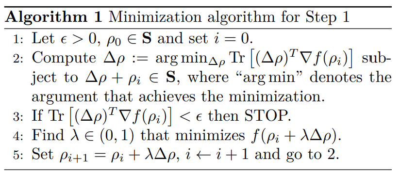
The notation is a little different, the differences are: their set \(S\) is my set \(E\), \(f(\rho) = S(\G(\rho)||\Z(\G(\rho)))\). Line 2 is simply the semidefinite program
\[\begin{aligned} \argmin_\omega & \sum_{j=1}^{n-m} \omega_j \tr(\Omega_j\T \nabla f(\rho_i)) \\ \st & \sum_{j=1}^{n-m} \omega_j \Omega_j + \rho_i \in \H^n, \end{aligned}\]
since the only free variable is \(\omega\), which is then used to construct \(\Delta \rho = \sum_{j=1}^{n-m} \omega_j \Omega_j\).
Step 2. Let \(\hat{\rho}\) be the minimising argument from Step 1, Step 2 starts with linearising \(S(\G(\rho)||\Z(\G(\rho)))\) about \(\hat{\rho}\). Due to numerical imprecision, \(\hat{\rho}\) actually corresponds to a slight upper bound on the minimum, but we want the calculated key rate to actually be achievable. So, Winick, Lütkenhaus, and Coles (2018) determine the dual problem to the linearisation, and maximise that, thus resulting in a solution which is a lower bound to the primal problem.
An open-source solver based on this method is available under the name Open QKD Security.
2.2 Example: BB84 protocol
This section will go through the first example in Appendix F of Winick, Lütkenhaus, and Coles (2018). The example follows the BB84 protocol described in Note 1, where Bob’s qubit detectors are not perfectly efficient. The experimentally determined constraints \(\Gamma\) will be modelled by a depolarizing channel (see Tip 1 for an explanation of a depolarising channel).
As described above, we know that Alice and Bob’s measurements of the qubits affect the state though the action of POVMs. Alice’s POVMs model whether or not Alice will measure a qubit in the \(z\)-basis, and are written as
\[\begin{aligned} & P_1^A = p_z \ket{0}\bra{0}, \ P_2^A = p_z \ket{1}\bra{1}, \ P_3^A = (1-p_z) \ket{+}\bra{+}, \\ & P_4^A = (1-p_z) \ket{-}\bra{-}, \end{aligned}\]
where \(p_z\) is the probability that Alice measures in the \(z\)-basis, and \(\ket{\pm} = \frac{1}{\sqrt{2}} (\ket{0} \pm \ket{1})\).
The state of a qubit can be visualised as being on the unit sphere, called the Bloch sphere in quantum mechanics.
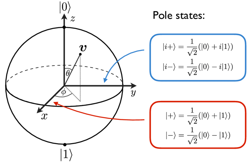
In the Bloch sphere diagram above, from Ketterer (2016), the \(x\)-, \(y\)-, and \(z\)-axes are labelled with their corresponding bases. The poles of the Bloch sphere correspond to \(\ket{0}\) and \(\ket{1}\), which are called the \(z\)-basis.
Alice’s system is modelled in qubits, but Bob’s system will be modelled in qutrits (three bits), to account for the possibility that the qubit Alice sends just doesn’t arrive, this is called a “no-click” event. Bob’s POVMs are
\[\begin{aligned} & P_1^B = p_z \ket{0}\bra{0} \oplus 0, \ P_2^B = p_z \eta \ket{1}\bra{1} \oplus 0, \ P_3^B = (1-p_z) \ket{+}\bra{+} \oplus 0, \\ & P_4^B \ket{-}\bra{-} \oplus 0, \ P_5^B = \one - \sum_{j=1}^4 P_j^B, \end{aligned}\]
where the \(\oplus 0\) indicates the addition of a third bit set to \(0\), and the factor \(\eta\) represents detector inefficiency. The fifth POVM is the one representing a no-click event, in this case the third bit is set to \(1\).
The depolarising channel, which represents the environmental effects on the qubits, is modelled by the Kraus operators \(\sqrt{1-\frac{3}{4}p} I\) (no change), \(\sqrt{\frac{p}{4}} X\) (bit flip), \(\sqrt{\frac{p}{4}} Y\) (bit flip with multiplication by \(i\)), and \(\sqrt{\frac{p}{4}} Z\) (phase flip), \(p\) is the depolarising probability. How the channel acts on a state is defined as
\[ \mathcal{E}(\rho) = (1-\frac{3}{4}p) \rho + \frac{p}{4}X \rho X^* + \frac{p}{4} Y \rho Y^* + \frac{p}{4} Z \rho Z^*.\]
This depolarising channel is used to simulate the experimental data by applying it to a maximally entangled state \(\ket{\phi}\) to generate \(\rho_\text{sim}\), which is then sampled by \(\Gamma_{jk} = P_j^A\otimes P_k^B\) to generate the \(\gamma_i\).
\[\begin{aligned} & \rho_{\text{sim}} = (I \otimes \mathcal{E})(\ket{\phi}\bra{\phi}), \\ & \gamma_{jk} = \tr((P_j^A\otimes P_k^B)\rho_{\text{sim}}), \end{aligned}\]
where \(I\) (by my understanding) is the identity acting on the no-click qubit of Bob’s state (Renner (2008)), \(\ket{\phi}\) is length \(6\), since a state vector of Alice and Bob’s joint state would be the tensor product of a state from Alice and a state from Bob, resulting in a length \(6\) vector.
Calculating the Kraus operators is a straight forward application of the equation given before, so we move on to the definition of the projection operator that determines which measurements of Alice’s and Bob’s to keep. We want to make sure that only the measurements where Alice and Bob measure in the same basis are kept, that is, Alice measures \(\ket{0}\bra{0}\) and Bob measures \(\ket{0}\bra{0}\) OR Alice measures \(\ket{1}\bra{1}\) and Bob measures \(\ket{1}\bra{1}\). The projector is written as
\[\Pi = \ket{0}\bra{0}_A \otimes \ket{0}\bra{0}_B + \ket{1}\bra{1}_A\otimes \ket{1}\bra{1}_B. \]
The last object to define is the isometry for the key map. It is defined such that Alice stores a 0 if she obtains outcome \(P_1^A\) or \(P3^A\), and stores a 1 if she obtains outcome \(P_2^A\) or \(P_4^A\), this is written as
\[ V = \ket{0}_R\otimes \ket{0}\bra{0}_A + \ket{1}_R\otimes \ket{1}\bra{1}_A,\]
where \(R\) is the register of key values.
With this, all components are defined to create the maps \(\G\), \(\Z\), and \(\Gamma\) for the optimisation problem in Equation 1.